In my MSc dissertation, I studied whether models trained on simulated microbial communities could infer parameters that explain real biological trajectories. Simulation gives us known parameters to learn from, but the real mouse microbiome data were sparse and noisy, and their underlying parameters were unknown, so I needed to test whether what the models learned in simulation remained useful under those conditions.
The Problem
I used the generalised Lotka-Volterra model, which describes how microbial populations grow and influence one another, to model eleven microbial taxa. Working backwards from observed population abundances meant estimating growth rates, directed interactions between every pair of taxa, and antibiotic susceptibilities, giving 143 parameters in total. These values cannot be read directly from an abundance curve, and the real dataset provided only nine mice divided across three intervention protocols.
The protocols covered a mostly stable control condition, exposure to clindamycin, and clindamycin followed by a C. difficile challenge, so the dataset allowed me to compare transfer in relatively stable communities with transfer when an external intervention changed the dynamics.
What I Built
-
I generated 12,000 synthetic ecologies, with nine trajectories for each ecology, giving 108,000 trajectories with different initial conditions and intervention histories.
-
To bring the training data closer to the real setting, I reproduced the mouse study’s sparse sampling schedules and included measurement noise, outliers, detection censoring, and explicit intervention events.
-
I kept each ecology within a single training, validation, or test split, so trajectories generated from the same parameter set could not appear on both sides of an evaluation.
-
Every neural model was trained and selected using synthetic data only, and I first evaluated its predicted parameters against the known simulation values.
-
For the real mice, where there was no parameter ground truth, I used the inferred parameters to simulate new gLV trajectories and compared those curves with the observations.
-
I also withheld one intervention condition at a time, so each model had to infer the system from the remaining mice before simulating a condition it had not observed.
Models and Evaluation
| Model family | What I compared |
|---|---|
| Classical baseline | Regularised gLV regression |
| Supervised inverse network | Parameter prediction from observed trajectories |
| Physics-informed inverse network | PINN with an equation-based constraint |
| Inverse operator | PI-DION with and without its physics residual |
| Quantum-classical variant | Hybrid quantum-classical PINN |
| Relational variants | Graph and attention-based decoders for species interactions |
The relational decoders predict interactions through relationships between species instead of treating the full interaction matrix as a single flat output.
I trained models across multiple random seeds, selected ensembles using synthetic validation data, and used paired bootstrap intervals when comparing methods, because an average from one run would not show how stable the differences were. I also included simple baselines, such as a persistence model that assumes the microbial population does not change. That baseline was difficult to beat on the nearly static control mice, so a low trajectory error there was not enough to demonstrate useful parameter inference.
What I Found
-
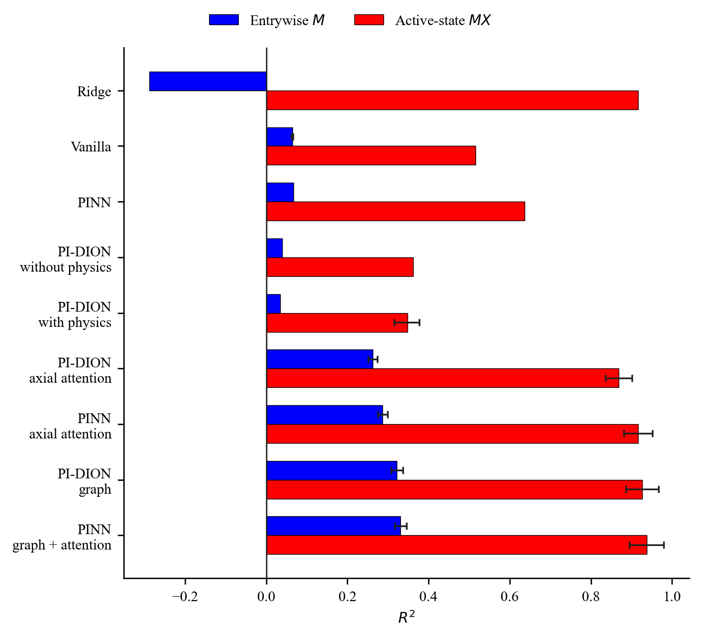
Synthetic recovery: recovering the interaction matrix was the main difficulty, and graph-based relational decoders reduced its recovery error by 21–28% relative to the standard PINN, supporting the use of species-to-species structure for this task.
-
Real-data transfer: every neural method achieved a lower mean trajectory error than Ridge across the six antibiotic-exposed mice, although none had received real-data weight updates. PINN graph plus attention performed best on those mice with the full cohort available, while PI-DION graph performed best on average when an entire intervention condition was hidden.
-
Physics constraint: in the matched PI-DION comparison, adding the equation residual lowered error on antibiotic-exposed mice by 2.2%, but worsened performance on the mostly static control mice and changed synthetic parameter error by less than 0.1%, so the benefit depended on the regime.
-
Quantum-classical model: it did not improve accuracy and required roughly 34 times the training time of the matched classical PINN.
Tools and methods
| Area | Tools and methods |
|---|---|
| Biological modelling | Generalised Lotka-Volterra dynamics, intervention-aware synthetic data |
| Neural models | PyTorch, PINNs, PI-DION, graph and attention-based decoders |
| Quantum variant | Hybrid quantum-classical PINN |
| Evaluation | Ecology-held-out splits, repeated seeds, paired bootstrap intervals, condition-held-out simulation |
What I learnt
No method performed best in every setting. Graph-based interaction decoders improved recovery on synthetic systems and transferred well to perturbed real mice, while the physics constraint helped only in particular regimes, so the choice of model needed to account for the dynamics being evaluated. The project also showed a practical limitation of synthetic-to-real learning, because the model that performs best on synthetic validation data may not transfer best to real data, and real parameter labels are unavailable to guide that selection.
Working through this benchmark helped me understand why evaluation design matters alongside architecture. Keeping ecologies separate, modelling realistic distribution shifts, including simple baselines, repeating seeds, and examining individual conditions allowed me to see where transfer was useful and where a favourable average could conceal a limitation.