I started this project to predict how a cell’s gene expression changes when a small molecule is applied to it, using compound structure and dose as inputs and the expression response as the output. Once the pipeline was working, I needed to understand whether differences between models were large enough to be measured against the noise in the data, so I extended the project into an audit of the benchmark itself.
The work runs on one laptop with an RTX 4050, 6 GiB of VRAM, 22 CPU threads, and 30 GB of RAM, without a cluster.
Main findings
- Most groups in the tested 24-hour sci-Plex panels had responses smaller than their estimated measurement error, so a pooled score could conceal how little headroom was available in much of the data.
- Model improvement was concentrated in the highest signal-to-noise quartile and in HDAC inhibitors, while molecular fingerprints did not demonstrate predictive value beyond mechanism-class labels in the tested comparisons.
- A five-seed paired comparison did not establish a statistically distinguishable difference between chemCPA and kernel ridge, although the first split had favoured chemCPA.
- The measurability finding also appeared on LINCS L1000, but that bulk dataset could not validate the relationship between single-cell sampling depth and the noise floor.
The sections below explain how I reached these conclusions and where the analysis remains limited.
Tools and methods
| Area | Tools and methods |
|---|---|
| Single-cell data | Scanpy, AnnData, streamed expression processing |
| Compound features | RDKit, Morgan fingerprints, ChEMBL |
| Predictive models | scikit-learn, PyTorch, Tanimoto neighbours and kernels |
| Benchmark evaluation | Compound-held-out splits, replicate noise floors, multi-seed comparisons |
| Protein features | ESM-2, shuffled-embedding and one-hot controls |
| Docking | AutoDock Vina, known-pose recovery checks |
Pipeline design and data preparation
The prediction pipeline
The prediction target is a control-relative pseudobulk response, which combines the single-cell measurements
within each (compound, dose) group into an average expression profile and subtracts a pooled control profile.
I use mean log-normalised counts averaged over two replicate plates and 1,000 genes selected from the training
data. Each compound is represented by a Morgan fingerprint (radius 2, 2048 bits) computed from its salt-stripped
parent structure, and I concatenate this with log10(dose) to include the exposure level.
I compare seven predictors on the same target: three non-learned baselines (zero response, training mean, and dose mean), a Tanimoto 5-nearest-neighbour model, ridge regression, a Tanimoto-kernel ridge with an RBF on log dose, and a small GPU MLP. I split the data by whole compounds, grouped on canonical parent structure, so different doses or salt forms of the same molecule cannot appear in both training and test data. Gene selection, scalers, and hyperparameter choice use training data only.
Before evaluating the models, I had to address three problems in the data preparation:
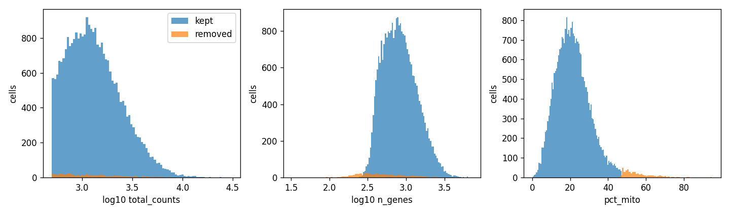
- A fixed 20% mitochondrial cut-off would have discarded 53% of cells, because these sci-Plex nuclei sit at roughly 20% mitochondrial reads by design, while an adaptive median+3·MAD cap removes 1.7% instead.
- Controls were being capped like treatments, which meant that every response in the first version was measured against a 30-cell mean, so I gave controls their own cap and balanced them across replicates.
- Compound naming silently dropped 36 of 188 compounds until I handled salt suffixes, after which all 188 resolved to 186 distinct parent structures.
Streaming the 2.5 GB expression matrix in chunks instead of subsetting it raised the usable cells per group from 36 to about 215 in 82 seconds, with 2.6 GB peak memory. This changed the main result without changing the model, which led me to investigate how much of the apparent model performance depended on the reliability of the measurements.
Measuring signal, replicate noise, and exposure effects
The measurement problem
Each (compound, dose) group is measured twice on separate plates, so disagreement between those replicates
provides an estimate of the measurement noise. I use this to estimate a floor for the error of the observed
two-replicate mean, against which model errors can be interpreted:
floor= RMSE(rep1 − rep2) / 2, the error of the observed two-replicate meansignal= sqrt(max(rms² − floor², 0)), the response magnitude with noise subtracted in quadraturesnr= signal / floor
Here, snr is the signal-to-noise ratio, and a value below 1 means that a group’s measured response is smaller
than its estimated measurement error.
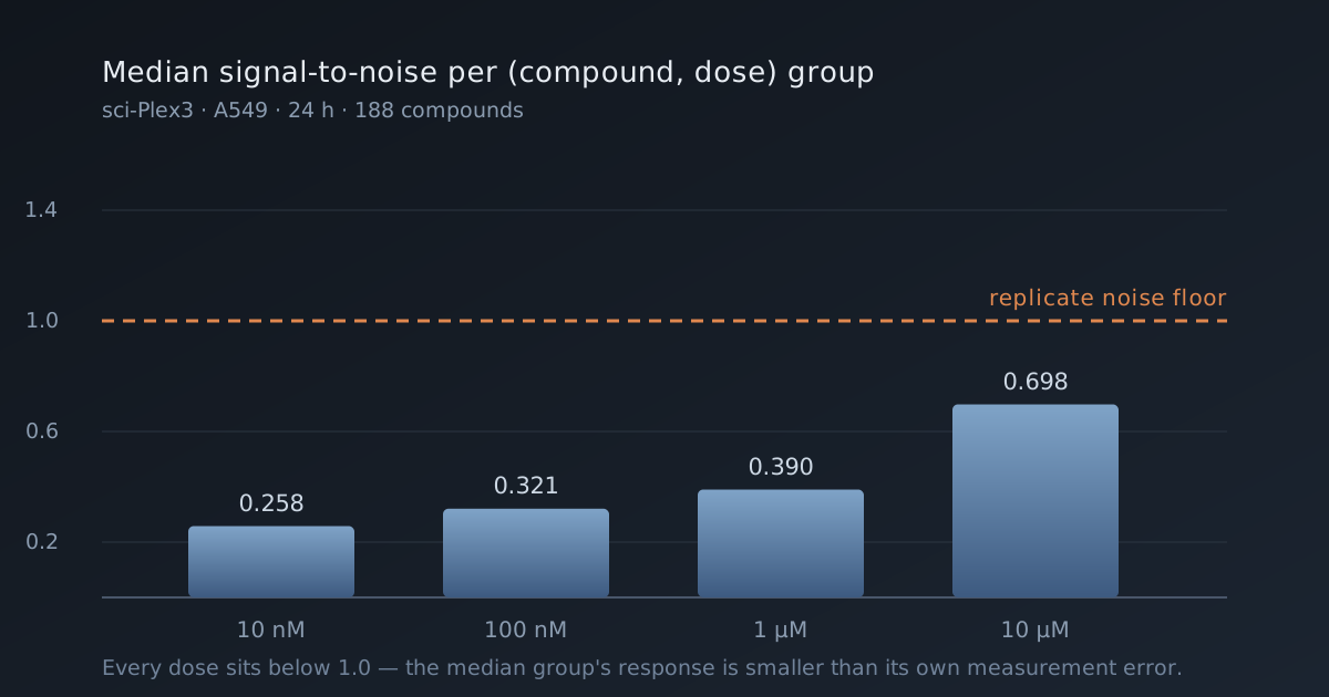
The median group is below 1 at every dose, in every 24-hour cell line tested:
| dataset | 10 nM | 100 nM | 1 µM | 10 µM | groups ≥ snr 1 at 10 nM | at 10 µM |
|---|---|---|---|---|---|---|
| A549 24 h | 0.258 | 0.321 | 0.390 | 0.698 | 8.0% | 39.9% |
| K562 24 h | 0.215 | 0.218 | 0.248 | 0.605 | 8.0% | 33.9% |
| MCF7 24 h | 0.000 | 0.000 | 0.345 | 0.619 | 8.0% | 39.9% |
| A549 72 h | 0.870 | 0.996 | 0.739 | 1.256 | 36.2% | 53.5% |
In MCF7 at the two lowest doses, the median noise-corrected signal is exactly zero, which means that the median group’s measured response is consistent with replicate noise under this estimate.
I had expected chemical specificity to be present at low dose and to weaken at high dose through off-target effects, but the measurements showed that low dose was the least measurable regime. Among the tested 24-hour conditions, appreciable signal was concentrated at the highest dose, so the results gave a practical reason for profiling at a high concentration even though that choice is often criticised.
Why the floor moves
To investigate what changed the floor, I regressed log(floor) on log(cells per group), obtaining slopes of
−0.543, −0.454, −0.354, and −0.421, compared with −0.5 for pure counting noise. Adding log dose raised R² by
at most 0.057 and produced a coefficient near zero, which supports sampling depth as the main explanation for
the noise floor. Dose can affect this indirectly when cytotoxicity reduces the number of surviving cells,
but the regression did not support a substantial additional dose effect after accounting for cell count.
Exposure time behaved differently: among the 47 compounds measured at both 24 and 72 hours, the 72-hour panel had 2.6× as many cells, predicting a sqrt(2.6) ≈ 1.6× reduction in the floor, close to the observed reduction of 1.63×. However, the snr gain reached 6.0×, which is larger than sampling depth alone can explain and supports an increase in signal with exposure. The comparison is conservative because this 47-compound subset was harder to measure at 24 hours than the full panel.
Model improvement by signal strength and dose
Where the models improve on the baselines
Because many groups had little measurable signal, I split the held-out groups into snr quartiles and
measured the fraction of the gap between the best non-learned baseline and the noise floor that each model
closed. This allowed me to check whether an improvement in the pooled score was shared across the dataset
or concentrated in the groups with stronger responses.
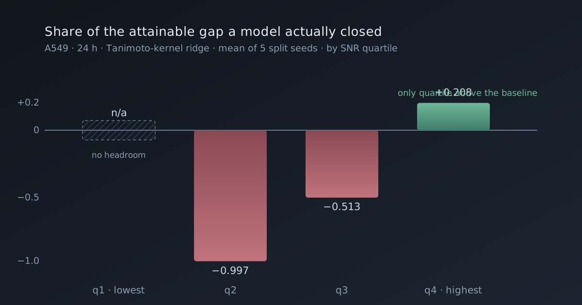
In the bottom quartile, the dose-mean baseline already sits below the replicate floor, so this measure provides no headroom in which to demonstrate an improvement. The models are substantially worse than that baseline in the second and third quartiles, while the top quartile is positive across the three cell lines, with values of +0.208 (A549), +0.216 (K562), and +0.187 (MCF7). Since RMSE gives greater weight to larger responses, the pooled result mainly reflects performance in that top quartile.
I then tested whether dose explained model improvement after accounting for measurability, by first
regressing per-group improvement on log dose alone and then adding snr to the regression:
| dataset | dose alone | dose given snr | 95% CI given snr | attenuation |
|---|---|---|---|---|
| A549 24 h | +0.00345 | −0.00154 | [−0.00345, +0.00008] | 144% |
| K562 24 h | +0.00354 | +0.00014 | [−0.00116, +0.00133] | 96% |
| MCF7 24 h | +0.00490 | +0.00014 | [−0.00138, +0.00159] | 97% |
| A549 72 h | +0.00370 | +0.00294 | [+0.00052, +0.00539] | 20% |
In the three 24-hour lines, the conditional dose coefficients weaken or change sign, their intervals include
zero, and adding dose to a model that already contains snr changes R² by only 0.000–0.003. This suggests that
the apparent relationship between dose and model improvement is largely explained by measurability in these
datasets.
A549 at 72 hours behaves differently, because its conditional dose coefficient remains positive and its interval excludes zero. This exception matters: the regression does not support treating measurability as a complete explanation of the dose relationship across every exposure time.
Testing molecular fingerprints against mechanism labels
Does chemical structure carry more than a class label?
A 2048-bit fingerprint describes molecular structure, while a 24-dimensional one-hot representation records only the mechanism class, such as whether a compound is an HDAC inhibitor. To test whether the structural information added predictive value beyond that label, I kept the compound split fixed on the true structures and changed the features, so every comparison held out the same molecules:
| model | A549 24 h | K562 24 h | MCF7 24 h | A549 72 h |
|---|---|---|---|---|
| Tanimoto-kernel ridge | +0.15 | +0.26 | +0.36 | +0.54 |
| Ridge | −1.25 | −0.83 | −1.14 | −0.13 |
| MLP | −1.73 | −1.07 | −0.67 | −1.18 |
The values are class_onehot − full fingerprint in units of the 5-seed standard deviation, so negative values
favour the one-hot representation. None of the twelve comparisons reaches 1 sd in favour of the fingerprint,
and the one-hot performs better in every dataset for ridge and the MLP. Fingerprints permuted within class or
globally perform worse than the real fingerprints in all sixteen comparisons, which shows that the real
features contain useful information, although these experiments do not demonstrate additional predictive
value beyond the mechanism label.
Looking at the mechanism classes separately showed that much of the expression improvement was concentrated in HDAC inhibitors, which account for about 16% of held-out groups and capture 29–33% of the attainable gap across the three cell lines. Other compounds capture 0.6–7.7%, and the K562 non-HDAC value is 0.006, effectively matching the dose-mean baseline. HDAC inhibitors also produce the largest responses in the panel, with snr 3.18 at the top dose, so their contribution is consistent with the relationship between model improvement and measurability.
Checking the conclusions with another evaluation metric
Checking the result with another evaluation metric
Since I constructed attainable_fraction for this analysis, I also needed to check whether the conclusion
depended on that particular metric. I scored every model using a Dynamic Range Fraction against an
interpolated duplicate positive control, both introduced by
Miller et al., whose paper argues that findings of deep models
losing to trivial baselines can arise from the evaluation metric. This provided a useful alternative way to
test whether the benchmark contained enough measurable variation for model improvements to be interpreted.
In the bottom three snr quartiles and at the lowest doses, the dynamic range is negative, because a technical duplicate, shrunk per gene according to its measured reliability, still cannot outperform the dose-mean prediction. The metric is undefined in these groups because there is no positive range to occupy, which supports the lack of demonstrable headroom found with my own measure.
The implementation retains their blending formula, but my weighting rule is different and is documented in
the code. Their weight is 1 − p_adj from a differential-expression test for each gene and condition, while
mine uses the per-gene reliability ratio s²/(s² + n²), which does not require a DE test and is the more
conservative of the two weighting rules. This is an adapted evaluation, not an exact reproduction of theirs.
The five-seed chemCPA comparison
Comparing chemCPA across multiple splits
chemCPA
(Hetzel et al., NeurIPS 2022) was a relevant model to compare, but its released checkpoints were fitted on a
split likely to contain my held-out compounds, so I retrained it from scratch to avoid that leakage risk.
Before training, I patched a project_folder symlink that pointed to the first author’s cluster path and an
on_train_end hook that called self.log() where Lightning forbids it, causing the final metrics to be
discarded after training completed.
On the first split, chemCPA had the lower error, at 0.1016 against 0.1071, but after recording that result I ran four more seeds to check whether the difference held across different sets of held-out compounds.
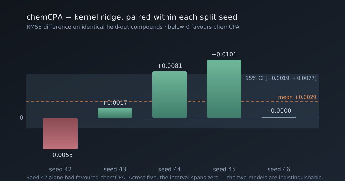
I paired the comparisons within each seed because the five held-out compound sets had only Jaccard 0.07–0.19 overlap. Across those pairs, the mean margin was +0.0029 in the kernel ridge’s favour, with a bootstrap 95% CI of [−0.0019, +0.0077]; chemCPA won 1 of 5 seeds, kernel ridge won 3, and one was a tie. The comparison did not establish a statistically distinguishable difference, and seed 42 was chemCPA’s best split of the five. Its apparent advantage in the top quartile was also unstable, with the margin changing sign in three of five seeds.
The same model’s error ranged from 0.1016–0.1247 across seeds as the held-out compounds changed, which was an order of magnitude larger than the mean difference between the models and larger than the paired margin’s standard deviation. This comparison showed why a single split was insufficient to rank these architectures on this benchmark. I marked the earlier single-seed conclusion as superseded in the repository and retained it so the reason for changing the conclusion remains visible.
Measurability on an independent platform: LINCS L1000
Testing measurability on LINCS L1000
Since sci-Plex has shallow sampling by construction, I checked whether the measurability result also appeared on LINCS L1000 Phase II, which measures bulk expression in a different laboratory and includes 1,750 compounds instead of 188, nine cell lines instead of three, and a median of three replicates instead of two. Before downloading 13 GB, I checked the metadata and found that 98,697 of 99,234 conditions had at least two replicates, so the replicate-based analysis was applicable to the data.
I analysed 76,397 conditions, referencing each condition to the vehicle controls on its own detection plate, and obtained the following measurability estimates:
| cell line | conditions | median snr | ≥ snr 1 |
|---|---|---|---|
| A375 | 10,881 | 0.000 | 8.2% |
| HT29 | 10,903 | 0.000 | 6.4% |
| MCF7 | 10,914 | 0.000 | 7.3% |
| HA1E | 10,876 | 0.000 | 6.0% |
| PC3 | 10,851 | 0.000 | 5.8% |
| YAPC | 9,361 | 0.000 | 4.1% |
| HELA | 9,358 | 0.000 | 3.8% |
| A549 | 1,625 | 0.243 | 16.3% |
| HEPG2 | 1,628 | 0.285 | 19.0% |
Median snr is 0.000 in seven of nine cell lines, and 74.4% of conditions have exactly zero noise-corrected signal, while only 6.5% exceed snr 1. The fraction above snr 1 also increases with dose, from 2.9% and 4.3% to 7.2% and 13.7% at 10 nM, 100 nM, 1 µM, and 10 µM respectively.
The proportion of conditions with little measurable signal is larger here than in sci-Plex, although A549 and HEPG2 have higher median snr values than the other cell lines. These two lines contain about 1,600 conditions each, compared with roughly 10,000 for the others, so their different sampling also needs to be considered when interpreting the exceptions.
This check supports the measurability finding and the ordering by dose, but it cannot validate the depth law,
because L1000 is bulk data and provides no cell count per condition with which to test 1/sqrt(cells).
The floor levels themselves are also not directly comparable (~0.42 against ~0.09), because the units and
preprocessing differ between platforms.
Independent checks on protein features and docking
Evaluating protein features and docking
I also evaluated frozen esm2_t6_8M_UR50D embeddings for 16 HDAC and kinase targets on a separate task,
predicting pChEMBL from Morgan fingerprints and a target representation across 88,011 compound–target pairs.
To check whether the embeddings contributed protein information or merely identified the targets, I included
a shuffled embedding control in which each target received another target’s vector:
| setting | no target | ESM | shuffled ESM | one-hot |
|---|---|---|---|---|
| scaffold split, all targets seen | 0.887 | 0.772 | 0.773 | 0.784 |
| leave-one-target-out | 1.188 | 1.142 | 1.282 | – |
When every target appeared in training, real and shuffled embeddings produced nearly identical errors (0.7724 against 0.7733) and performed similarly to a one-hot, so this setting did not demonstrate useful protein information beyond a target label. When a target was held out, real embeddings beat the shuffled control on 13 of 16 targets, supporting some transferable signal, although the margin was small and strict leave-one-target-out R² remained negative for every variant.
Before interpreting docking predictions, I tested whether the workflow could recover known poses. Across 170 runs, benzamides redocked successfully in their own structures with top-1 success 0.95, while hydroxamates never ranked a correct pose first, even in their native receptor, although a correct pose was sampled in 70% of runs and zinc was engaged in 100%. This points to a scoring limitation rather than an inability to sample the pose: Vina does not explicitly model the zinc chemistry needed to favour bidentate chelation, so I label those rankings as weak evidence wherever they appear.
Limitations and what I learnt
This project helped me understand how measurement quality limits what can be concluded from a model comparison. Much of the tested chemical perturbation data had insufficient signal relative to replicate noise, while sampling depth and exposure time helped explain measurability, and the structural features did not demonstrate predictive value beyond mechanism class in the tested comparisons. I also examined alternative explanations involving dose-dependent mechanisms, magnitude saturation, cytotoxic selection, a noise ceiling, and detection and composition effects, rather than assuming that every weak model result had the same cause.
-
Two evaluation choices I made also proved misleading, and I retained them in the record with explanations. The within-class fingerprint scramble preserves class membership but replaces real chemical similarity with noise of similar magnitude, so it can weaken the class signal instead of isolating sub-class structure as I had intended.
-
An initial stratified chemCPA comparison used the minimum over seven of my models in each stratum, which selected on noise and introduced a bias worth 0.00017 pooled but 0.01685 in the top quartile, larger than chemCPA’s entire advantage there. This made chemCPA appear worse in every quartile when it was better in all of them, showing why the comparison rule itself needed checking.
-
The depth relationship still needs external validation on single-cell data at a scale this machine cannot process, so it remains a next experiment rather than a result replicated by the L1000 analysis.
Code, tests and every result table cited here are at github.com/ruman-shaikh/Cell2Compound.